


Optimization of a centrifugal compressor impeller using CFD: the choice of simulation model parameters
V V Neverov, Y V Kozhukhov, A M Yablokov, A A Lebedev
Abstract. Nowadays the optimization using computational fluid dynamics (CFD) plays an important role in the design process of turbomachines. However, for the successful and productive optimization it is necessary to define a simulation model correctly and rationally. The article deals with the choice of a grid and computational domain parameters for optimization of centrifugal compressor impellers using computational fluid dynamics. Searching and applying optimal parameters of the grid model, the computational domain and solver settings allows engineers to carry out a high-accuracy modelling and to use computational capability effectively. The presented research was conducted using Numeca Fine/Turbo package with Spalart-Allmaras and Shear Stress Transport turbulence models. Two radial impellers was investigated: the high-pressure at ѱT=0.71 and the low-pressure at ѱT=0.43. The following parameters of the computational model were considered: the location of inlet and outlet boundaries, type of mesh topology, size of mesh and mesh parameter y+. Results of the investigation demonstrate that the choice of optimal parameters leads to the significant reduction of the computational time. Optimal parameters in comparison with non-optimal but visually similar parameters can reduce the calculation time up to 4 times. Besides, it is established that some parameters have a major impact on the result of modelling.
Introduction
The design quality of the flowpath is one of the basic factors that determine the overall efficiency of centrifugal compressors. Automatic optimization techniques are used for the aerodynamic and mechanical design of turbomachine components. The optimization algorithm based on a sequence of 3D simulations for a large number of stage shape variations, which are generated to improve output parameters, as efficiency, pressure ratio, head etc. There are many approaches to optimization, which are good for optimal solution search [1]. Therefore, proper problem definition, the selection of the main parameters and criteria for optimization allows designers to significantly improve the performance of the final product [2].
Most computational fluid dynamic software packages include the full-cycle optimization algorithm with geometrical model parameterization, geometry and mesh regenerating tools. This allows CFD users to easily use geometric CFD optimization software to automatically generate design variants. These software packages often include a built-in optimization algorithm (in most cases it is genetic algorithm) or have the ability to use third-party code, as IOSO. Thus, technical aspects is well understood at the moment, and it is not problem to realize a sequence of calculations.
Despite the many advantages, their use is usually limited to simple applications in industrial practice, because of their high computational cost. During optimization computing systems work through many variants of a flowpath to achieve the desired result. If a powerful cluster with hundreds of cores carries out the calculations [3], the efficiency of optimization will not drop. This will increase only the workload of computing machine and the cost of electricity. In the case of low-power computing systems, performance of the works and the manufacture of products will be reduced. For this reason, one of the main problem that an iteration of optimization takes long time to compute. Therefore, one of the methods of increasing the optimization effectiveness is to decrease the time per one iteration while keeping the adequacy of calculation results. In this way, efficiency of the optimization mostly depends on the accuracy of the simulation model [4].
- The aim of study and the object of research
The aim of the study is to investigate the influence of the computational domain and mesh model parameters on the integral parameters of the impeller and the rate of obtaining a converging solution. The best combination of these parameters will be used for future multiobjective optimization.
In this study, computation models of two radial impellers of the centrifugal compressor with cylindrical blades have been used:
The first one is a low-pressure impeller (IMP1) with the mean-camber curve of the blade formed by a circular arc. The flow rate coefficient F=0.06; the Euler work coefficient ψT=0.43; the impeller exit diameter is 0.82m; blade outlet angle βbl2=32°; the number of blades z=13.
The second one is a high-pressure impeller (IMP2) impeller with the mean-camber curve of the blade formed by an s-shaped curve. The flow rate coefficient F=0.064; the Euler work coefficient ψT=0.71; the impeller exit diameter is 0.4m; blade outlet angle βbl2=75°; the number of blades z=24.
Mesh model generation and subsequent computations were carried out using Numeca Fine/Turbo. The Fine/Turbo is a specialized CFD suite for rotating machinery with incompressible and compressible fluids that proved oneself as the fastest, accurate and convenient tool [5].
The computational domain and variations of the inlet and outlet boundary are shown in figure 1. The following boundary conditions were applied: steady conditions, air ideal gas as fluid, total pressure and temperature as inlet boundary condition, mass flow as outlet boundary condition. The following two turbulence models were compared: Spalart-Allmaras and Shear Stress Transport. Furthermore, the regions of labyrinth seals were not included in the computational model to speed up the calculations. The values of the polytropic efficiency presented below was corrected for estimated losses of the disk friction and leakage through labyrinth seals.
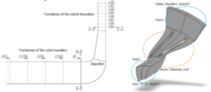
Figure 1. Control sections and computational domain variations
The polytropic efficiency, which were calculated at cross-sections 0-0 (impeller inlet) and 2-2 (impeller exit) shown in figure 1.The following were taken as a result of calculation:
- The number of iterations required to reach the convergence. The calculation were considered as converging when flow variables, which was monitoring at inlet and outlet boundaries, reach a steady-state value and the mean-squared residuals are dropped by four orders.
- The non-dimensional time per one iteration (normalized by a minimum time per one iteration in each series of calculations).
- The non-dimensional computing time required to reach the convergence (normalized by a minimum computing time in each series of calculations).
In general, the time per one iteration depends on the mesh size and the number of processor cores used in calculations. The computing time depends on both the number of iterations to reach convergence and the time per one iteration. In present paper, the overall computing time is considered as the main evaluation criteria.
- The influence of the outlet boundary location
The flow separation and the so-called “trace” after impeller blades may have a significant impact on computational results if the outlet boundary is defined close to the impeller exit. The study was conducted with fixed inlet boundary by extending the part of the vaneless diffuser where width b3=b2. The overall number of mesh elements is increased in conjunction with the number of elements in vaneless diffuser. The computational domain and locations of the outlet boundary are shown in figure 1. To determine the efficiency, the flow parameters were derived from sections 0-0 and 2-2 (=1.05D2). The calculation results for both impellers are shown in figures 2 and 3.
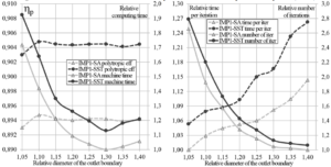
Figure 2. The influence of the outlet boundary location for the low-pressure impeller (IMP1)
For the low-pressure impeller, the difference between obtained efficiencies for different location of the outlet boundary is small, and at 1.15D2 efficiency approaches a constant value. The number of iterations to reach convergence, which is described by the power-law function, is reduced while the outlet boundary is located at the range from 1.05D2 to 1.3D2. However, placing the outlet boundary further away from the section 2’-2’, increases the total number of elements and the time per one iteration. Thus, from the point of view of computing time, the optimal location of the outlet boundary is at 1.3D2. Further shifting of the outlet boundary from section 1.3D2 is useless, because the number of iterations is not reduced and the time per 1 iteration is increased.
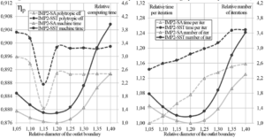
Figure 3. The influence of the outlet boundary location for the high-pressure impeller (IMP2)
In case of the high-pressure impeller, the location of the outlet boundary has a strong impact on the integral parameters because heterogeneity of the flow behind blades is greater than that in the low-pressure impeller. For that reason alone, to calculate a high-pressure impeller it is necessary to place the outlet boundary at least at 1.25D2. On the other hand, according to calculation results the convergence deteriorated after 1.2D2. The number of required iterations for the SA turbulence model is increased by a factor of 2.3 when the outlet boundary is shifted from 1.2D2 to 1.4D2. This is due to the separated flow in the elongated sections of the diffuser, which leads to pulsations of the mass flow at the outlet boundary and slows down the convergence of the calculation. In figures 2 and 3, the width of the diffuser is equal to the width of the channel at the exit of the impeller, i.e., b3/b2=1. Increasing of the diffuser width contributes to the emergence of the separated flow in a diffuser. Therefore, in addition to the original case b3/b2=1, the case b3/b2=0.8 has been considered. Based on calculation results, narrowing of the diffuser had no effect. If the outlet boundary is placed at the distance greater than 1.2D2, the convergence deteriorates in comparison with the original case. Therefore, the most appropriate option is to locate the outlet boundary at 1.25D2, where the solution can be considered acceptable and the convergence rate is not critically increased.
To sum up, the influence of the outlet boundary location is as follows:
For the high-pressure impeller, the outlet boundary location has significant impact on result of the numerical experiment. In comparison with the low-pressure impeller, to reach the convergence more iterations and, therefore, greater computing time is needed because the flow is more heterogeneous. In the range from 1.05D2 to 1.2D2 number of required iterations is reduced by factor of 1.4. If the diameter of the outlet boundary is greater than 1.25D2, the convergence deteriorates due to the separated flow and the unsteady phenomena in the vaneless diffuser.
For the low-pressure impeller, the effect of the outlet boundary location is relatively small; the convergence improves by elongation of the diffuser. As a result, in the presented case, computing time was reduced by more than 1.7 times. However, the effectiveness of the elongation is limited by the optimal ratio of the required number of iterations and the time per one iteration.
For all series of calculations, following should be noted: the calculation under SA turbulence model reaches convergence faster by 10-20% than under the SST model, which is consistent with the fact that the SST model is more complicated. Similarly, the time per one iteration is smaller by 5-15% than that for the SST model. The SST model exhibits the polytropic efficiency overestimation by 0.5-1% in absolute values in comparison with the SA model. This difference was also observed in other studies of the centrifugal compressors using Numeca Fine/Turbo [6]. In General, the performance curves for both turbulence models are equidistant.
- The influence of the inlet boundary location
The location of the inlet boundary is often chosen randomly. It can also be based on the geometric shape of section before impeller, but at the same time, the inlet chamber or the return channel of the previous stage is not considered. However, the choice of the long entrance section could not be reasonable. The influence of the inlet chamber or the return channel of the previous stage could be preset by velocity, pressure and temperature profiles at the inlet boundary. But it brings its own problems in the implementation. Otherwise, setting the uniform field does not simulate the real flow in the inlet section, and therefore the rationality of increasing the grid model by extending the inlet section is not obvious. In order to save up computational power, the optimal location of the inlet boundary should be chosen.
The search of the optimum length of the entrance section in front of the impeller were conducted in the range from 0 to 0.75D2. The calculation results are shown in figures 4 and 5.
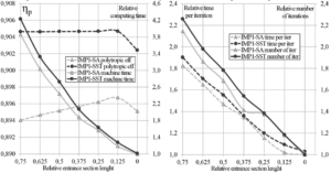
Figure 4. The influence of the inlet boundary location for the low-pressure impeller (IMP1)
For the low-pressure impeller, decreasing of the entrance length led to the linear increase of efficiency under the SA turbulence model and to the constant efficiency under the SST model. The sharp drop of the efficiency by 0.2% occurs for both used turbulence models at the zero length. This drop is due to the fact that the velocity profile at this location already changed to enter impeller blades and it is different from the preset profile by the uniform field on this coordinate. It changes the flow around blades and leads to the difference in efficiency of impeller. Therefore, in spite of the continuing acceleration of the convergence, the choice of a short entrance section is precarious.
In General, the location, where the velocity profile is significantly changed, depends on many factors (for example: the width of the impeller, the length of the section under the shroud labyrinth seal, smoothness of the meridional turn and difference between areas at sections 0-0 and blade inlet 1-1).
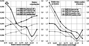
Figure 5. The influence of the inlet boundary location for the high-pressure impeller (IMP2)
The high-pressure impeller has longer system of the labyrinth seals provided by design than the low-pressure impeller. Therefore, under the zero length of the entrance section, the velocity profile does not have an impact on flow around the leading edge, but it is resulted in a sharp deterioration of the convergence. The main factor that accelerate the convergence is reduction in the total number of mesh elements as described further. Thus, if the inlet chamber or the return channel of previous stage are not simulated, then it is pointless to choose long entrance section along with increasing the size of the grid. For both considered impeller the optimum inlet boundary is located at 0.125D2.
- The influence of the mesh parameters
4.1. Mesh topology
The choice of the grid dimension for verification of the numerical experiments is solved by the standard examination of the grid independence. This study allows us to determine the number of mesh elements, starting from which increasing this number have no effect on calculation results. As for the optimization problem, it is reasonable to choose grid parameters more accurate, providing acceptable calculation results with minimal time spent on solving. Mesh generator Numeca AutoGrid 5 allows user to generate block-structured parameterized mesh. In the automatic mode for the radial impeller, it is usually possible to use two kinds of topology: O4H and H&I. O4H is a default topology composed by 5 blocks: an O block around the blade, 2 H-blocks upstream the leading and trailing edges of the blade and 2 H-blocks up and down to the blade section. The H&I topology is often used to obtain better mesh quality with multiblades configuration. The H&I topology is composed by: one block to mesh the blade passage, contrary to the default topology which creates a mesh around the blade; an optional skin block around the blade with two H-blocks before and after the skin block. The difference between grids with both topologies is shown in figure 6. In contrast to the O4H type, the grid-type H&I uses an intersectoral splitting with boundary near the blade surface. This splitting may lead to less intensive convergence due to averaging associated with a periodic boundary condition.
In general, the choice of the mesh topology is based on a grid model quality: the minimum skewness of the elements, the maximum expansion ratio of adjoining elements, etc. Therefore, both topologies cannot be right for all configurations of impellers. If it is possible to generate mesh for both topologies that equivalent in quality, it is reasonable to choose topology be guided by the speed of solution obtaining. The mesh generated using both topologies was calculated and compared. The number of total grid elements for both impellers (IMP1 and IMP2) is 1.15 million, the minimum skewness for IMP1 — 45°, IMP2 — 36°. The time per one iteration for both topologies is the same, because the numbers of mesh elements are equal. The required number of iterations are presented in Table 1.
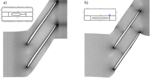
Figure 6. a) O4H mesh topology; b) H&I mesh topology (overall mesh size 1,15 million)
| Table 1. Results of the calculation under mesh topologies | ||||||||
| IMP1 | IMP2 | |||||||
| Turbulence model | SA | SST | SA | SST | ||||
| Mesh topology | O4H | H&I | O4H | H&I | O4H | H&I | O4H | H&I |
| Number of required iteration | 696 | 835 | 830 | 1022 | 1070 | 1305 | 1390 | 1606 |
Thus, the optimal choice of the mesh topology allows to save up to 20% of computing time that is encountered when carrying out a large number of calculations.
- Mesh refinement
Research on grid independence is a standard procedure for conducting a various numerical experiments. Findings of such researches are shown in many articles, for example [7].
The size of general mesh element is decreased with the total number of mesh elements increasing. The error that can be quantified by mesh refinement is known as the discretization error. Using an optimal mesh, the accuracy of the results are good enough to capture all the necessary flow features, their gradients and so forth. For both investigated impellers, the optimal number of elements were chosen for further optimization calculations. The result for the low-pressure impeller are shown in figure 7. The result for the high-pressure impeller correspond with result for the low-pressure impeller.
Starting with 0.8 million elements the efficiency of the low-pressure impeller almost ceases to change. The time per one iteration grows linearly and the number of required iteration is almost linear. As a result, the computing time required to reach convergence is described by non-linear function and it is considerably increases when the number of the mesh cells exceeds 1 million elements. Therefore, the optimal size of the mesh is the size that lies in the range of cell quantity from 0.8 to 1 million for one blade sector. This mesh size range for this impeller is good enough to achieve acceptable accuracy at the expense of minimum possible computational power. For the high pressure impeller the optimal number of elements is about 0.6-0.8 million, because this impeller has smaller size, larger number of blades and consequently smaller blade passage than the low-pressure impeller.
-
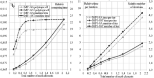
Figure 7. The influence of the number of mesh elements for the low-pressure impeller (IMP1)
The mesh parameter y+ is a non-dimensional distance between the first node and the wall. This parameter is important for the turbulence model selection (Low-Reynolds or High-Reynolds), because it determines the requirement to the grid. Under High-Reynolds models with standard wall-function, it is necessary to avoid values of y+ less than about 20-30 and greater than 300 for the calculation of the gas flow. Whereas under Low-Reynolds models with scalable wall functions, the recommended range of y+ is from 0.001 to 1, because using scalable wall functions requires to have a sufficiently thin layer of elements to decompose the boundary layer. A trial calculation is usually carried out to determine y+ in the whole computational domain. Then the size of the first near-wall cell is corrected manually to meet the criterion. The influence of this parameter considered in article [8].у+ parameter
It is believed that Low-Reynolds models allow to predict points of local separations more accurate, however, such models make high demands on the grid dimension. In present paper Low-Reynolds models were used. The influence of the parameter y+ is considered in the recommended range (from 0.001 to 1) and out of it (from 1 to 48) on integral parameters and the rate of convergence (see figure 8 and table 2).
| Table 2. Variation of the cell height and values of the parameter y+ | |||||||||
| Variations | 1 | 2 | 3 | 4 | 5 | 6 | 7 | 8 | |
| IMP1 | Height of cell, mm | 0.001 | 0.0015 | 0.005 | 0.01 | 0.03 | 0.08 | 0.15 | 0.3 |
| Average y+ | 0.17 | 0.25 | 0.82 | 1.75 | 5.5 | 12.6 | 19.7 | 30.4 | |
| Maximum y+ | 0.59 | 0.86 | 3.03 | 6.23 | 14.6 | 25.2 | 34.5 | 47.7 | |
| IMP2 | Height of cell, mm | 0.0005 | 0.0007 | 0.0012 | 0.005 | 0.01 | 0.03 | 0.08 | 0.15 |
| Average y+ | 0.12 | 0.165 | 0.276 | 1.17 | 2.5 | 7.3 | 16.0 | 24.4 | |
| Maximum y+ | 0.38 | 0.53 | 0.92 | 4.08 | 7.8 | 16.1 | 28.1 | 39.9 | |
As can be seen in figure 8, the y+ in the recommended range does not have any noticeable effect on the convergence. That is, in this range the rate of convergence remains constant. Increasing in the average value of the parameter y+ from 0.17 to 0.82, efficiency of the low-pressure impeller is increased by 0.5% and then at y+=1.75 is dropped by 0.7%. For the high-pressure impeller results are similar.
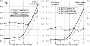
Figure 8. The influence of the parameter y+ for the low-pressure impeller (IMP1)
Increasing of the parameter y+ out of the recommended range leads to an incorrect results, when the efficiency of the impeller increased. It is arise from the significant decrease of friction losses, because of the insufficient resolution of grid dimension in the boundary layer. Along with incorrect results, the number of iteration is significantly increased. With the equal time required per one iteration, the computing time is increased in proportion to the required number of iterations. In case of the high-pressure impeller, integral parameters and the convergence rate are correspond to those for the low-pressure impeller. However, the SST model makes exacting requirements for the y+ parameter: at y+>2.5 the calculation was interrupted. Thus, the interruption of the calculation under the SST model may be due not only to the overall quality of the mesh, but also due to an unacceptably large size of the first near-wall cell. In this case, under the SA model it is possible to reach the convergence, even at a significant deviation from the recommended range.
- Potential saving of the computing power
To sum up, the optimization of investigated impellers under optimal and random parameters of the computational model gave the following results:
The random parameters: the inlet boundary located at 0.5D2, the outlet boundary located at 1.1D2; the selected grid topology is H&I; the height of near-wall cell is 0.01 mm (which is corresponding to the average value of y+=1.75); the total number of cells – 1.15 million.
The optimal parameters: the inlet boundary located at 0.125D2, the outlet boundary located at 1,3D2; the selected grid topology is O4H; the height of near-wall cell is 0.001 mm (which is corresponding to the average value of y+=0.17); the total number of cells – 0.92 million.
According to the result of the calculation, under non-optimal parameters, the time per one iteration on a single processor core was 3 seconds and the number of required iterations to reach the convergence was 775. Consequently, the total computing time of calculation for a single approximation of the optimization was 2322 seconds. As for calculation under optimal parameters, these values are respectively equal to 2.4 seconds per iteration and 227 iterations. Moreover, the total calculation time was 535 seconds, which is faster than the calculation with non-optimal parameters by 4.25 times. Thus, 100 optimization steps would be taken 64 hours under randomly chosen parameters and 15 hours under optimal parameters. This is a significant difference, considering the fact that computational domains and mesh models are visually similar for both variants.
Conclusion
As a result, presented research reveal the most important parameters of the computational model (the location of the outlet boundary and the overall size of the grid) during large series of calculation. These parameters with non-optimal values, regardless of the impeller type, increase the time of obtaining converging solutions by 2 times or more and have a significant influence on results of calculation (up to 1.7% of impeller efficiency for the outlet boundary and 1.5% for the grid model). This is unacceptable when optimizing the geometric shape of impellers in case of both adequacy result and the rational use of computing resources.
Besides, to obtain adequacy result, the grid parameter y+ for selected turbulence models and the location of the inlet boundary should be observed. For the Low-Reynolds turbulence models, too large values of the grid criterion y+ have the significant impact on the calculation result.
According to results of a preliminary assessment, optimal parameters of the computational model were determined. For the low-pressure impeller IMP1 – the outlet boundary is defined at 1.3D2; the inlet boundary located at 0.125D2; mesh topology is O4H; the size of the near-wall cell is 0.002 mm; the total number of grid elements is 0.9 million. For the high-pressure impeller IMP2 – the outlet boundary is defined at 1.25D2; the inlet boundary located at 0.125D2; mesh topology is O4H; the size of the near-wall cell is 0.001mm; the total number of grid elements is 0.7 million. These sets of computational model parameters provide the optimal computing time while keeping adequacy of results. Thus, determined values may be considered as a reference point to define a computational model of 2D-impellers. However, it is necessary to check overall quality of the computational model in each individual case.
References
- Frese F, Einzinger J, Will J 2012 Design optimization of an impeller with CFD and Meta-Model of optimal Prognosis (MoP) 10th International conference of turbocharges and turbocharging 2012, London, pages 121-134
- Dickmann H P 2013 Shroud contour optimization for a turbocharger centrifugal compressor trim family 10th European Turbomachinery Conference (Lappeenranta, Finland)
- Boldyrev Y, Rubtsov A, Kozhukhov Y, Lebedev A, Cheglakov I, Danilishin A 2015 Simulation of unsteady processes in turbomachines based on nonlinear harmonic NLH-method with the use of supercomputers CEUR Workshop Proceedings Volume 1482, Pages 273-279
- Galiando J, Hoyas S, Fajardo P, Navarro R 2013 Set-up analysis and optimization of CFD simulations for radial turbines Engineering Applications of Computational Fluid Mechanics, 7(4), 441-460. doi: 10.1080/19942060.2013.11015484
- Borm O, Kau H-P, Unsteady aerodynamics of a centrifugal compressor stage–validation of two different CFD solvers 2012 Proceedings of ASME Turbo Expo 2012, GT2012, Copenhagen, Denmark, June 11-15, GT2012-69636
- Borm O, Balassa B, Kau H-P Comparison of different numerical approaches at the centrifugal compressor radiver 2011 ISABE Conference, International Society for Airbreathing Engines, Gothenburg, Sweden, 12th-16th September 2011 ISABE-2011-1242
- Le Sausse P, Fabrie P, Arnou D, Clunet F 2013 CFD comparison with centrifugal compressor measurements on a wide operating range EPJ Web of Conferences, Vol. 45, p. 01059
- Aghaei Tog R, Tousi A M, Tourani A 2008 Comparison of turbulence methods in CFD analysis of compressible flows in radial turbomachines Aircraft Engineering and Aerospace Technology 80, Iss. 6, Pages 657-665 ISSN 1748-8842